Rasterizing Shapefiles in R

2014/ 05/15

I recently needed to convert a shapefile to a raster for use in another package and wanted to share my steps here.

For this demonstration, I started with the Natural Earth Data 1:10m Physical Vectors Land

shapefile and will convert it to a raster using the raster package.

A bit of searching around on the web led me to Amy Whitehead’s page on Converting shapefiles to rasters in R . The code listed there wasn’t quite what I needed but gave me the head start on figuring out what I needed to do.

Load required packages

The maptools package is used to import the shapefile to a SpatialPolygonsDataFrame and the raster package is for rasterizing the shapefile.

library(maptools)

## Loading required package: sp

## Checking rgeos availability: FALSE
##      Note: when rgeos is not available, polygon geometry     computations in maptools depend on gpclib,
##      which has a restricted licence. It is disabled by default;
##      to enable gpclib, type gpclibPermit()

library(raster)

Load the shapefile we’ll be rasterizing

Use the readShapePoly function from package maptools to read our shapefile in as a SpatialPolygonsDataFrame.

# Retrieved from http//www.naturalearthdata.com/download/110m/physical/ne_110m_land.zip
shape_url <- "http://www.naturalearthdata.com/http//www.naturalearthdata.com/download/110m/physical/ne_110m_land.zip"
shape_folder <- tempdir()
shape_path <- tempfile(tmpdir = shape_folder, fileext = ".zip")
download.file(shape_url, shape_path)
unzip(shape_path, exdir = shape_folder)
dir(shape_folder)

##  [1] "devtools4bf4152fc28f"
##  [2] "devtools4bf431284c83"
##  [3] "devtools4bf4334c9928"
##  [4] "devtools4bf4355aa26c"
##  [5] "devtools4bf46278c6fd"
##  [6] "devtools4bf468d5df12"
##  [7] "devtools4bf47558b59"
##  [8] "devtools4bf48790d1c"
##  [9] "downloaded_packages"
## [10] "file4bf429c8b448"
## [11] "file4bf43b4c949f"
## [12] "file4bf4411676aa"
## [13] "file4bf4434bad9c"
## [14] "file4bf45ea45e1b.zip"
## [15] "file4bf4617ac199"
## [16] "file4bf4d7ffb4b"
## [17] "libloc_213_722ad5f9e07c7fe1.rds"
## [18] "ne_110m_land.cpg"
## [19] "ne_110m_land.dbf"
## [20] "ne_110m_land.prj"
## [21] "ne_110m_land.README.html"
## [22] "ne_110m_land.shp"
## [23] "ne_110m_land.shx"
## [24] "ne_110m_land.VERSION.txt"
## [25] "repos_https%3A%2F%2Fcran.rstudio.com%2Fbin%2Fmacosx%2Fel-capitan%2Fcontrib%2F3.5.rds"
## [26] "repos_https%3A%2F%2Fcran.rstudio.com%2Fsrc%2Fcontrib.rds"
## [27] "Rprofile-devtools"
## [28] "rs-graphics-0cee3d3c-f7dd-4e3f-b7e7-548de668efab"

land <- readShapePoly(file.path(shape_folder, "ne_110m_land.shp"))

## Warning: readShapePoly is deprecated; use rgdal::readOGR or sf::st_read

Create a blank raster

Before we can rasterize the shapefile, we need to create a blank raster. We specifiy the number of rows and columns to control the spatial resolution of our raster. We also have to specify the spatial extent, which will determine how much of the area of our shapefile we’re rasterizing. Here, I use the extent function from the raster package to grab the extent of the shapefile and pass that to the raster function. You can also specify extent manually.

blank_raster <- raster(nrow = 100, ncol = 100, extent(land))

If we were to plot this now, we would get an error because, by default, new rasters are created without any values. Rasters are fundamentally just like a 2-dimensional matrix (though they are stored as 1-d vectors). To get at this 2-d matrix, rasters have a slot

called data, which you can access by calling blank_raster@data. You can get (and set) the values of the raster using the values function.

values(blank_raster) <- 1
plot(blank_raster)

Above, we’ve set all those values to 1 and the result is just a raster of one value (color). The values inside the raster are stored in a vector of length nrow * ncol, so let’s set the values equal to the sequence of numbers from 1:nrow*ncol.

values(blank_raster) <- 1:(100*100)
plot(blank_raster, col=rainbow(50))

Pretty cool! So we can see that raster’s values are stored going from the top-left to the bottom-right.

Rasterize the shapefile

The first line here is pretty straightforward but the second line requires some explanation. The raster function tries to assign values to the resulting raster cells. Cells inside any of the polygons of the shapefile will have some value, while cells not included in any of the polygons of the shapefile will have the value NA. For some shapefiles, values are picked up from the attributes embedded in the shapefile and will result in variation in values (colors). In my case, I want to force all cells corresponding to land to be equal to 1 and leave the rest NA.

land_raster <- rasterize(land, blank_raster)
land_raster[!(is.na(land_raster))] <- 1

Plot the result

Rasters can be plotted directly with the plot function because the raster package implements its own plot method. Here, we also add the shapefile back on top of the raster to see how we did.

plot(land_raster, legend=FALSE)
plot(land, add=TRUE)

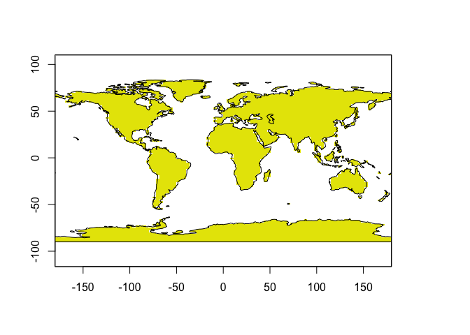
Looks pretty good! The filled-in yellow area is the new raster. Let’s zoom in to see what’s going on.

plot(land_raster, legend=FALSE, xlim=c(-170, -120), ylim=c(30, 65))
plot(land, add=TRUE,  xlim=c(-160, -120), ylim=c(30, 90))

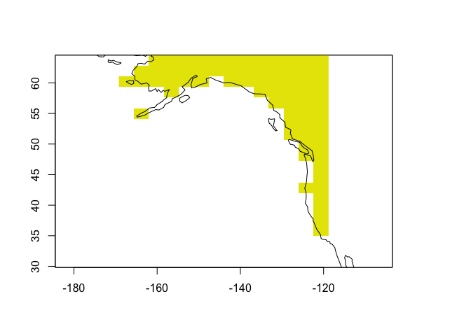
Not great. The raster cells are roughly outlining the land but end up being pretty poor approximations in places. Clearly, we might like to improve the spatial resolution of our raster but this is a pretty good start.

Let’s the spatial resolution up to see if we can do better.

blank_raster <- raster(nrow = 1000, ncol = 2000, extent(land))
land_raster <- rasterize(land, blank_raster)
land_raster[!(is.na(land_raster))] <- 1
plot(land_raster, legend=FALSE, xlim=c(-170, -120), ylim=c(30, 65))
plot(land, add=TRUE,  xlim=c(-160, -120), ylim=c(30, 90))

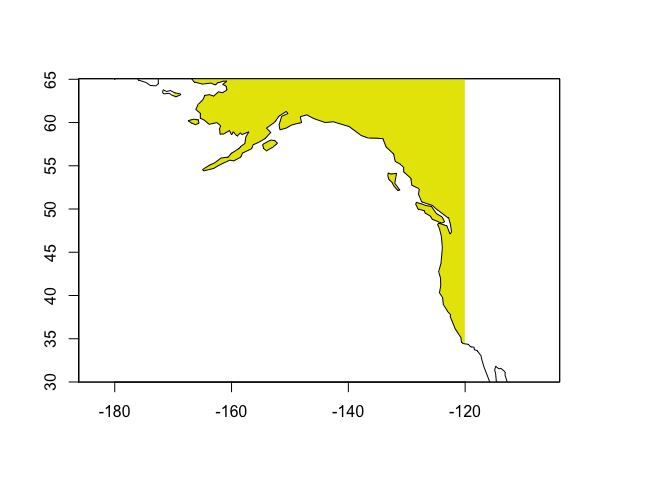
Much better!

Bonus: Effect of different raster resolutions

In the above example, I used a 100x100 grid for the raster. Below, I test 20x20, 100x100, 500x500, and 1000x1000 grids together to explore the effect of that part of the process. What resolution do we need to adequately describe the shape of the land?

layout(matrix(1:4, ncol=2, byrow=TRUE))

resolutions <- c(20, 100, 500, 1000)

for(r in resolutions)
{
  blank_raster <- raster(nrow = r, ncol = r, extent(land))
  land_raster <- rasterize(land, blank_raster)
  land_raster[!(is.na(land_raster))] <- 1

  plot(land_raster, legend=FALSE, xlim=c(-170, -120), ylim=c(30, 65), main=paste0("Resolution: ", r, "x", r))
  plot(land, add=TRUE,  xlim=c(-160, -120), ylim=c(30, 90))
}

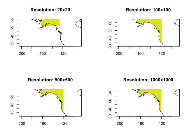
You can see that, by 500x500, we’re getting a raster that looks pretty close to the underlying shapefile.