Working with NetCDF files in R

2014/ 02/18

NetCDF is an open file format commonly used to store oceanographic (and other) data such as sea surface temperature (SST), sea level pressure (SLP), and much more. I recently needed to work with SST data from the NCEP Reanalysis and found that I didn’t know how to work with NetCDF files. This post should serve as a short introduction working with NetCDF files using the R package ncdf.

Step 1: Acquire the NetCDF library

Before we can open a NetCDF file in R, we need to install the NetCDF library on our system. I’m using a Mac running OS 10.9 and I use homebrew as my package manager.

If you’re using homebrew, install the netcdf library with:

brew install netcdf

If you’re on Windows, you can find pre-built binaries at the developer’s download page. For other systems, consult the documentation.

Step 2: Install and load the `ncdf` package in R

install.packages("ncdf4")

And load it:

library(ncdf4)

Step 3: Load your NetCDF file

For this tutorial, I’ll be working with the NOAA Optimum Interpolation (OI) Sea Surface Temperature (SST) V2 data series of monthly means from December 1981 – current. These data are produced on a 1° grid for the entire globe.

sst_url <- "ftp://ftp.cdc.noaa.gov/Datasets/noaa.oisst.v2/sst.mnmean.nc"
sst_path <- tempfile()
download.file(sst_url, sst_path) # 53.0 MB
cdf <- nc_open(sst_path)

I am interested in the following variables: latitude, longitude, time, and SST:

lat <- ncdf4::ncvar_get(cdf, varid="lat")
lon <- ncdf4::ncvar_get(cdf, varid="lon")
time <- ncdf4::ncvar_get(cdf, varid="time")
sst <- ncdf4::ncvar_get(cdf, varid="sst")

The lat and lon variables are just vectors containing the range of latitudes (89.5S to 89.5N) and longitudes (0.5°E to 359.5°E, starting from the prime meridian).

The time variable is a little more complex. Let’s take a look:

head(time)

## [1] 66443 66474 66505 66533 66564 66594

Those don’t look like times at all. If you’re used to working with dates and times on computers, you may already be way ahead of me. If, however, if you are not, I’ll explain. Dates and times are usually stored by computers as a number of time units since we started counting time. The time units may be milliseconds, seconds, or even months – whatever suits the purpose. Computers commonly store dates and times as the number of seconds since January 1, 1970 (See UNIX time ). In the case of our data, time is being counted as days since January 1, 1800. This is a little weird but it makes sense for our data. If you’re using a different NetCDF file than me, you’ll want to consult the documentation that goes along with the data to figure out how they’re counting time.

Now that we know how time is being stored, we can make it human-readable:

time_d <- as.Date(time, format="%j", origin=as.Date("1800-01-01"))
time_years <- format(time_d, "%Y")
time_months <- format(time_d, "%m")
time_year_months <- format(time_d, "%Y-%m")

Here, I set the origin to January 1, 1800 and then convert the original variable time into a vector of R Date objects, passing the parameters format="%j" and origin=as.Date("1800-01-01"). The time variable is now much more easier to understand:

head(time_d)

## [1] "1981-12-01" "1982-01-01" "1982-02-01" "1982-03-01" "1982-04-01"
## [6] "1982-05-01"

The other variables I created, time_years, time_months, time_year_months are for added utility. I can now reference SST data for just a set of years

time_years %in% c("1990", "1991")

or all SST values from June

time_months %in% c("06")

Our last, but most important variable is SST.

dim(sst)

## [1] 360 180 441

sst is three dimensional, and is indexed by longitude, latitude, and time (respectively). To extract a single SST value from it, we’ll need to specify an index or range of indices for all three dimensions:

sst[lon==220.5, lat==50.5, time_d==as.Date("1990-06-01")]

## [1] 10.91

We can use our utility variables to, for example, extract all the observations for June from this same grid cell:

sst[lon==220.5, lat==50.5, time_months=="06"]

##  [1]  9.27 10.25  9.68  8.81  9.75  8.96  8.82  9.79 10.91 10.04  9.55
## [12] 11.01 10.55  9.46  9.39 10.21 10.00  7.94  9.39  8.78 10.08 10.05
## [23] 10.56 10.67  9.78  8.65  8.33 10.04  8.88  9.11  8.21 10.19 11.51
## [34] 12.05 10.27  9.76 10.32

Depending on your goals, this may be as far as you need to get. But maybe you want to display these data visually. Let’s plot the SSTs for a range of grid cells onto a map.

Step 4: Convert the SST data to a `data.frame`

Our NetCDF file has a lot of observations:

prod(dim(sst))

## [1] 28576800

To reduce the amount of computation, let’s subset the data to a range of latitudes and longitudes and also focus in on a particular month in the data set so we can plot this in two dimensions:

lat_range <- seq(55.5, 60.5)
lon_range <- seq(190.5, 195.5)

lat_indices <- lat %in% lat_range
lon_indices <- lon %in% lon_range
time_indices <- time_year_months=="1990-06" # June of 1990

Notice how I constructed the _indices variables. They are vectors of the same length as their corresponding variable but they contain TRUEs and FALSEs where the corresponding variable is equal to the desired ranges. This allows instant subsetting:

sst[lon_indices, lat_indices, time_indices]

##      [,1] [,2] [,3] [,4] [,5] [,6]
## [1,] 4.20 4.12 4.63 5.47 6.19 6.63
## [2,] 4.39 4.05 4.40 5.18 5.99 6.64
## [3,] 4.71 4.04 4.11 4.73 5.58 6.55
## [4,] 5.21 4.39 4.32 4.82 5.63 6.61
## [5,] 5.57 4.91 4.80 5.17 5.87 6.70
## [6,] 5.53 5.36 5.29 5.55 6.12 6.81

Which gives us the SST values for the 5x5 grid for June of 1990. To save them in a more convenient format, we’ll convert it to a data.frame.

cdf_df <- expand.grid(lat_range, lon_range)
names(cdf_df) <- c("lat", "lon")
cdf_df$sst <- NA
head(cdf_df)

##    lat   lon sst
## 1 55.5 190.5  NA
## 2 56.5 190.5  NA
## 3 57.5 190.5  NA
## 4 58.5 190.5  NA
## 5 59.5 190.5  NA
## 6 60.5 190.5  NA

Now each row of cdf_df will correspond to one SST value, one row for every grid cell combination (25 in total). Let’s populate it with SST values:

for(i in 1:nrow(cdf_df))
{
  lat_ind <- which(lat == cdf_df[i,"lat"])
  lon_ind <- which(lon == cdf_df[i,"lon"])

  cdf_df[i,"sst"] <- sst[lon_ind, lat_ind, time_indices]
}

head(cdf_df)

##    lat   lon  sst
## 1 55.5 190.5 6.63
## 2 56.5 190.5 6.19
## 3 57.5 190.5 5.47
## 4 58.5 190.5 4.63
## 5 59.5 190.5 4.12
## 6 60.5 190.5 4.20

Looks good! Let’s make a map to display these data on. Luckily, this is pretty straightforward in R using the maps and mapdata packages.

library(maps)
library(mapdata)
map('world2Hires', xlim=range(lon_range) + c(-10, 10), ylim=range(lat_range) + c(-5, 5))
box()
points(cdf_df$lon, cdf_df$lat)

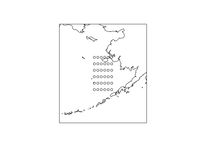
The above map is a good start. I’ve used the world2Hires map from mapdata which lets me create a map centered on the Eastern Bering Sea. I’ve specific the x- and y-limits to show just the area where we have SST values. Let’s change the points to rectangles and make the background color of the rectangles correlate with the corresponding SST value for that grid.

We’ll first make the color scale:

ncolors <- 5
cols <- cut(cdf_df$sst, ncolors)
palette <- colorRampPalette((c("blue", "red")))(ncolors)

To plot rectangles instead of points, we can use the rect() function instead of points(). rect() draws rectangles on the graphics device and needs the user to specify the coordinates of each corner (xleft, ybottom, xright, ytop).

map('world2Hires', xlim=range(lon_range) + c(-10, 10), ylim=range(lat_range) + c(-5, 5))
box()

grid_hw <- 0.5 # Grid half width
rect(cdf_df$lon - grid_hw, cdf_df$lat - grid_hw, cdf_df$lon + grid_hw, cdf_df$lat + grid_hw, col=palette[cols])

map.axes()
title(main="June SST Values", xlab="Longitude", ylab="Lattitude")
legend("topright", legend=levels(cols), fill=palette)

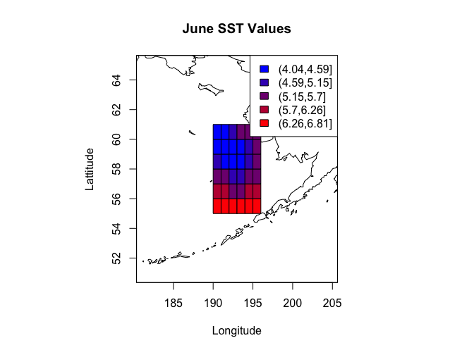
Looks great! Hopefully this post was a useful introduction to working with and displaying NetCDF data.